M14 1s-orbital

Louis de Broglie first proposed in 1924 that electrons have wave properties.
The energy E of a light-photon is proportional to its frequency :

Using Einstein’s formula (E=mc²), de Broglie formulated the following equation for the wavelength of an electron:

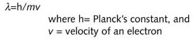
This equation has the form :

Wave property = Constant / Particle property

Thus, de Broglie assigned both particle-properties and wave-properties to the electron. Later, in 1926, Erwin Schrodinger used this model in a differential equation which expressed the wavelike characteristics of the electron.

Solutions to Schrodinger’s wave equation can be obtained only under certain conditions, which represent certain well-defined electronic states. We can understand this physically as follows: if an orbiting electron is treated as a wave, then to avoid destructive interference an integral number of wavelengths must be fitted into one circuit.
Solving this wave equation for the electrons of the hydrogen atom gives a series of wave functions. Each wave function, , corresponding to a particular energy level of the electron and its position. Each wave function actually describes an atomic orbital.

The intensity of a wave is proportional to the square of its amplitude. The wave function , is an amplitude function. is proportional to the electron density or the probability P of the electron at each point in space. The probability that the electron can be found at a particular point is proportional to the density of a charge cloud at that point.

For an electron in the n=1 state, or a 1s-orbital, the electron density has its maximum near the nucleus and is reduced to zero at the core. Beyond this maximum the density decreases as the distance from the core increases.
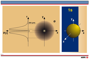
The diagram on the left of illustration M14 is the radial probability P(r) curve i.e. the probability of finding an electron at a given distance from the core.

In the middle of illustration M14 a contour diagram is shown (= cross-section of the electron charge cloud) for the 1s-orbital. The dashed line at about 200 pm from the nucleus delimits the region with a probability of 90%. There is a 90% chance that the electron is to be found in the region between the core and this fictive limit. On the right a boundary surface representation of the 1s-orbital is shown. A surface is obtained by joining the points of equal probability with one another. This encloses a volume in which there is a 90% chance of finding an electron.